Plus article on lottery

The UK National Lottery began on 19th November 1994 and by 20th October 2007 there had been 1240 draws. The jackpot prize is won by choosing in advance the 6 numbers to be drawn from a set of balls numbered from 1 to 49. The lottery illustrates many aspects of the theory of probability. Each draw is individually unpredictable, yet the overall history shows predictable patterns. A `league table' of numbers can be created that appears to show some numbers are preferentially drawn, and yet the table is completely spurious; how to test whether the balls are truly being drawn at random; how extremely unlikely events will occur if you wait long enough, and so on.

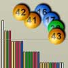
Starting from 1994, note how the 'leader' changes, until one number seems to gain a substantial lead.

If you click on 'Show histogram', you can create the current distribution of how often each of the 49 numbers has come up. The distribution seems quite spread out, with some numbers appearing much more often than others, but in fact this apparent spread should be purely due to chance. National Lottery - Level 2 considers what sort of distribution of total appearances of each number we would expect, when lottery balls are chosen at random.

What about the gaps between numbers?

Full Screen Version

Using the animation above, work backwards from October 2007 and see how long you have to wait until the last number appears. Do you think this is surprising? We can use probability theory and simulations to explore how long we have to wait for a number to come up.

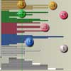
The animation below shows the gap between each time a number comes up - click on the link LottoRuns.swf to run it in full screen.

Can you see the longest gap that has occurred? Look carefully from the start of 2000. Do you think this is surprising? National Lottery - Level 2 considers what sort of gaps between numbers we would expect when lottery balls are chosen at random.

National lottery - Level 1 shows how many times each of the numbers has come up in the main National Lottery draw, and what were the gaps between appearances of each number. Here we look at whether the observed distribution of the number of times each of the 49 numbers has come up fits with what would be expected with a truly random draw, and whether the gaps also correspond to what might be expected.

The number of appearances of each number

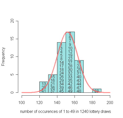
If the lottery balls are being chosen at random, then the distribution of the number of times each ball comes up should follow the theoretical shape shown when you click on 'Show theoretical' - click on the link Lotto2 to run it in full screen..

Of course the actual distribution is more jagged, but the theoretical distribution allows us to see whether the 'leading' number is surprisingly far in front. Below we see the final observed distribution with an approximate theoretical distribution superimposed. The fit looks good, suggesting, as we would expect, that there is no systematic preference for particular numbers.

In National Lottery level 3 we consider some of the mathematics behind the theoretical distribution of counts, and how to check if the observed distribution is in conflict with the theoretical one.

Are the gaps what we would expect?

If you run the animation below, then if the lottery balls are being chosen at random, then the distribution of the gaps should follow the theoretical shape shown when you click on T (NB not currently available). This theoretical distribution is known as a Geometric distribution and is derived in National Lottery - Level 3.

After 1242 lottery draws, with 6 main balls being drawn each time, $6\times 1242 = 7452$ numbers have been drawn, and so there are 7452 gaps between two draws of the same number (the gaps until the first time each number is drawn are included in this total). The histogram below shows the distribution of all these 7452 gaps, with the theoretical geometric distribution superimposed. The gaps are divided into those below and above 40, so that the large gaps are clearly displayed: the theoretical distrbution seems to fit the observed distribution well, although there are inevitably some jagged bits in the tail.

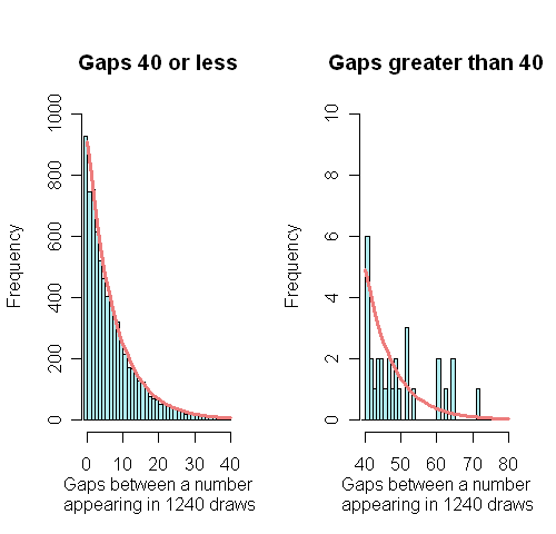
The longest gap observed is 72, for number 17 , which appeared on draw 435 on 23rd February 2000, but did not appear again until draw 508 on 4th November 2000. How surprising is it to get a gap as large as this? After a specific occurrence of a particular number, this is extremely surprising, and there is only 8/100000 chance of such an extreme result. However, when we take into account that there were 7452 gaps observed and this was the largest one, it turns out that it is not surprising at all. In fact 72 is almost exactly the average maximum gap one would expect in a series of 1242 lottery draws!

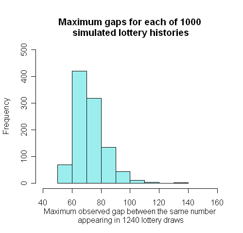
Alternatively we can use the power of the computer to simulate 'fictional' lotteries, by picking 6 different numbers at random from 1 to 49, and then repeating this process as long as we want. The software contains 'random number generators' that should ensure that each number really does have an equal chance of being chosen. We simulated 1000 full lottery histories and found the longest gap in each history. These 1000 longest gaps had the distribution shown below: 420 out of 1000 were 72 or more.

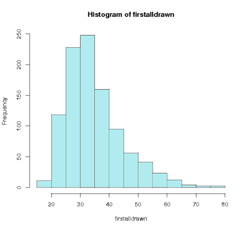
As another example of using simulations, looking backwards from 20th October 2007, we saw that ball 14 was not drawn until the 53rd draw. The graph below shows the results of simulating 1000 lotteries until all the numbers had come up. In 60 of these simulations we had to wait until at least 53 draws before all the numbers had come up, showing the time we had to wait for ball 14 was not really very surprising.

In National Lottery level 3 we consider the mathematics behind the theoretical distribution of gaps.

In National Lottery Level 2 we looked at the observed and theoretical distributions for the total count of times each number has come up, and the gap between a number's appearances. Here we explain the mathematics behind the theoretical distribution of counts, and how to check for true randomness, and derive the theoretical distribution for gaps.

The distribution for the number of times each number has been drawn

We first need to introduce some notation. Let the number of balls chosen at each draw be $m=6$, and the number of balls in the 'bag' be $M=49$. Each number between 1 and 49 therefore has a $p=m/M=6/49$ chance of being chosen at a particular draw. Therefore after $D$ draws, the total number of times each ball has been drawn has a Binomial distribution with parameters $p$ and $D$.

This distribution has mean $Dp$ and variance $Dp(1-p)$, and can be approximated by a Normal distribution with matching mean and variance. This is what is done in the animation.

Testing for bias in the lottery

There are many test statistics that are designed to identify different ways in which the lottery draws may not be entirely random, such as favouring odd or even numbers and so on (Haigh, 1997). We consider the simplest possible: an adapted chi-square test.

After $D$ draws, we expect any particular number $j$ to have occurred $E_j = Dp = Dm/M$ times, whihc in the UK lottery corresponds to $6D/49 \approx D/8$ So, for example, after 1000 draws we would expect each number to have been chosen around 125 times. If after $D$ draws we add up the total number of times each number has occurred, and label these totals $O_1,...,O_{49}$, then a naive chi-squared statistic compare the observed and expected counts using the standard formula
$$ X^2_{\rm naive} =\sum_{j=1}^{j=M} \frac{(O_j - E_j)^2}{E_j},$$
which would be compare to a theoretical $\chi^2$ distribution with $M-1=48$ degrees of freedom. For those not familiar with chi-squared tests, this statistic will be large if the observed counts are very different from the expected, since then the numerators $(O_j - E_j)^2$ will be very big. However we would never expect the observed to exactly match the expected, due to chance variation, and it turns out that if the numbers really are drawn at random then the statistic should be approximately 48, if we assume all the balls being drawn were statistically independent.

However, as Haigh (1997) points out, this would only be the case if all $mD$ individual ball-draws were independent, which is not the case as 6 balls are drawn without replacement at each lottery-draw. Hence it is impossible, for example, for a particular number to be drawn as ball 2 and 6 within a single draw. This lack of independence requires an adjustment to the chi-squared statistic above, so that the correct statistic is
$$ X^2 = \frac{(M-1)}{(M-m)}X^2_{\rm naive};$$
hence the adjustment factor multiplies the naive chi-squared statistic by a factor 48/43 $\approx$ 1.12. This adjusted statistic is shown in the lottery animation.

If we group the lottery draws in sets of 50, we can plot the $X^2$ statistics for successive groups. This is shown below, with the lower and upper 2.5\% points of a $\chi^2_{48}$ distribution drawn in, respectively 30.8 and 69.0.

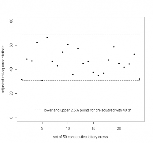
We see that all the 24 statistics lie inside the central 95\% interval for the $\chi^2_{48}$ distribution.

The distribution of gaps between a number's appearances

Suppose a specific number $j$ has just been drawn. Then suppose that we label successive draws a ‘success’ if $j$ is drawn, a ‘failure’ otherwise: the chance of a ‘success’ is defined as $p$ which in this case is 6/49. Let $X$ be the number of failures before the first success, i.e. the ‘gap’ before $j$ is drawn again. The chance of a $X=0$ is the same as the chance of $j$ appearing in the next draw, which is $p = 6/49 \approx 0.12$. The chance of a gap of 1 is the same as the chance of a single 'failure' and then a 'success', which is $(1-p)p = 43/49 \times 6/49 = 0.11 $, and so on. Therefore the chance of $X$ taking on any particular value $x$ is the same as the chance of observing a series of $x$ ‘failures’ followed by a single ‘success’, so that
$$ {\rm Pr}(X=x) = (1-p)^x p.$$
This is the Geometric distribution: note that sometimes this distribution is defined as the time until the first success, which here corresponds to $Y=X+1$. The mean of this distribution is $1/p - 1 = 49/6 – 1 = 7.16$, so the average gap length is around 7.

The maximum gap in the whole lottery history

We observed a maximum gap of 72 for ball number 17 between February and November 2000, which seems extraordinarily long. Is this surprising?

The chance of any particular gap being at least $x$, ie ${\rm Pr}(X \ge x)$, is simply the chance of observing $x$ failures in a row, so that
$${\rm Pr}(X \ge x) = (1-p)^x.$$
Therefore the chance of observing a gap as long as 72 is $(43/49)^{72}$ = 0.000082 , or around 1 in 12,500, which seems very rare indeed. If after number 17 was drawn in February 2000, we had specifically said 'let's wait until 17 appears again', then we would have been justifiably mazed at having to wait 73 draws until it did appear again, and might even suspect it had been left lout of the bag! However we did not pre-specify this particular gap as being interesting, and simply chose it as the largest of 7452 observed gaps. Therefore a crude estimate of such a rare event occurring, when there are 7452 opportunities for it to occur, is $0.00082 \times 7452 = 0.61$. A more accurate estimate is obtained by noting that, if there are $n$ independent gaps,
$${\rm Pr( maximum-gap }\ge x) = 1- {\rm Pr( maximum-gap }< x) = 1- {\rm Pr( all-gaps }< x) = 1- {\rm Pr}( X < x) ^n = 1- [1-{\rm Pr}( X \ge x)] ^n,$$
since the probability that all gaps are less than $x$ is the product of $n$ identical probabilities that a single gap is less than $x$. Hence we would estimate the probability of a maximum gap being at least 72 as $1 - (1 - 0.000082)^{7452} = 0.46$. This result suggests that 72 is not in the least surprising.

However, as with the $\chi^2$ statistic above, this distribution theory is not quite correct as there is some dependence between the gaps induced by there being exactly 6 numbers selected at each draw. We can therefore conduct a simulation with the results shown before and reproduced below.

In 1000 simulations of 1242 draws, the mean largest gap was 72 , 154 was largest gap, 42% were 72 or more (showing the approximation assuming independence, 0.46, is quite accurate). Therefore our maximum gap of 72 is almost exactly what one would expect.

National Lottery Level 4 will (probably) derive the adjusted chi-squared statistic and do other clever stuff.

Further reading and links

This is based on an idea by Fenton on considering the lottery results as a league table.

A spreadsheet with the full lottery history can be downloaded from the main UK National lottery site

This discussion is primarily based on Haigh (1997) whose notation we use.

Haigh J (1997) The statistics of the National Lottery. J R Statist Soc A, 160, 187-206.